Samplers and schedules

Open in Colab View on GitHub DownloadGPU

A trained diffusion model only tells us, for a noisy image, what it thinks the clean image is. A sampler turns that into a picture: it starts from pure noise and takes a series of steps down the noise levels. Notebook 01 writes DDIM, Euler, DDPM and Heun by hand. Here we take the flower model trained in notebook 02 and run every sampler Dew ships on it, at a few step counts, from the same starting noise, and time each one.

Run notebook 02 first, in the same folder: this notebook loads its checkpoint from runs/02-diffusion. It expects one NVIDIA GPU and took about two minutes on an RTX 4080.

Install

%pip install -q "dew-ml[cuda13] @ git+https://github.com/AshishKumar4/dew"

Note: you may need to restart the kernel to use updated packages.

Settings

STEP_COUNTS are the numbers of noise levels each sampler walks. SAMPLES is how many images each run draws.

import os

IMAGE_SIZE = 64
CHECKPOINT = "runs/02-diffusion"
STEP_COUNTS = [10, 20, 40]
SAMPLES = 4
SEED = 0

# The tutorial test sets DEW_TUTORIAL_SMOKE=1 to run every cell in minutes on a CPU.
if os.environ.get("DEW_TUTORIAL_SMOKE") == "1":
    STEP_COUNTS, SAMPLES = [2, 4], 2

import time

import jax
import jax.numpy as jnp
import matplotlib.pyplot as plt
import numpy as np

print(jax.devices())

[CudaDevice(id=0)]

Loading the trained model

A checkpoint holds arrays, not code, so we first rebuild the model and the objective exactly as notebook 02 built them. A Trainer over the same objective and the same checkpoint folder then restores the latest step with place(). We only want the weights, so the optimizer here never takes a step.

import optax
from dew import Checkpoints, Field, InputSpec, Trainer, models, presets
from dew.objectives.diffusion import DiffusionObjective

process = presets.EDM()()
model = models.build(
    "simple_dit",
    patch_size=4,
    emb_features=256,
    num_layers=6,
    num_heads=4,
    output_channels=3,
    dtype="bfloat16",
    attention_impl="auto",
)
objective = DiffusionObjective(model, process, InputSpec(Field("image", (IMAGE_SIZE, IMAGE_SIZE, 3))), ema_decay=0.999)
state, _, _ = Trainer(objective, optax.adamw(3e-4), key=jax.random.key(0),
                      checkpoints=Checkpoints(CHECKPOINT)).place()
print("restored step", int(state.step))

Resumed from step 6000 in /tmp/nbwork/run/runs/02-diffusion
restored step 6000

The same starting noise for every sampler

To compare samplers fairly, everything except the sampler has to stay fixed. We draw the starting noise $x_T$ once and hand the same array to every run. The ancestral samplers (DDPM and Euler ancestral) also add fresh noise at every step; sample derives that noise from the key we pass, and we pass the same key every time.

x_T = process.noise(jax.random.key(SEED), (SAMPLES, IMAGE_SIZE, IMAGE_SIZE, 3))
print("x_T spread:", float(jnp.std(x_T)))

x_T spread: 80.20647430419922

The samplers

DDPM follows the reverse Markov chain of the original DDPM paper and adds fresh noise at every step. It needs many small steps.
DDIM is the deterministic version: jump to the next noise level along the direction the model points to.
Euler takes one Euler step of the probability-flow ODE per noise level. On this schedule it is the same update as DDIM written differently.
Euler ancestral takes an Euler step to a slightly lower level and then adds back some fresh noise, so it solves the reverse SDE instead of the ODE.
Heun takes an Euler step, asks the model again at the end of it, and averages the two slopes. That costs two model calls per step.
RK4 is classical fourth-order Runge-Kutta: four model calls per step.
MultiStepDPM reuses the model’s answers from the last three steps to correct the current one, at one model call per step.

Each is a small value in dew.sampling. As in notebook 02, process.denoiser(model, params, {}) wraps the model and its weights into the function a sampler calls, and sample(denoise, x_T, steps, solver=..., key=...) runs any of the samplers over it in one loop.

from dew.sampling import DDIM, DDPM, RK4, Euler, EulerAncestral, Heun, MultiStepDPM, sample

SOLVERS = {
    "DDPM": DDPM(),
    "DDIM": DDIM(),
    "Euler": Euler(),
    "Euler ancestral": EulerAncestral(),
    "Heun": Heun(),
    "RK4": RK4(),
    "MultiStepDPM": MultiStepDPM(),
}

To time the samplers fairly we compile each one once with jax.jit and time only a second call. The step count and the solver are static arguments, so every combination compiles its own loop. The weights are a normal argument, which keeps them out of the compiled program.

import functools

@functools.partial(jax.jit, static_argnames=("steps", "solver"))
def run(params, x_T, key, steps, solver):
    denoise = process.denoiser(model, params, {})
    return sample(denoise, x_T, steps, solver=solver, key=key)

params = objective.trainable(state.averaged)
images, seconds = {}, {}
for steps in STEP_COUNTS:
    for name, solver in SOLVERS.items():
        run(params, x_T, jax.random.key(SEED), steps, solver).block_until_ready()
        start = time.perf_counter()
        out = run(params, x_T, jax.random.key(SEED), steps, solver).block_until_ready()
        seconds[name, steps] = time.perf_counter() - start
        images[name, steps] = np.asarray(out)

One grid per step count. Each row is a sampler and each column one starting noise, so images in the same column started from the same point.

def show_grid(steps):
    figure, axes = plt.subplots(len(SOLVERS), SAMPLES, figsize=(SAMPLES * 1.1, len(SOLVERS) * 1.1))
    for row, name in enumerate(SOLVERS):
        for column in range(SAMPLES):
            axis = axes[row, column]
            axis.imshow(np.clip((images[name, steps][column] + 1) / 2, 0, 1))
            axis.set_xticks([])
            axis.set_yticks([])
        axes[row, 0].set_ylabel(name, rotation=0, ha="right", va="center", fontsize=8)
    figure.suptitle(f"{steps} steps")
    plt.show()

for steps in STEP_COUNTS:
    show_grid(steps)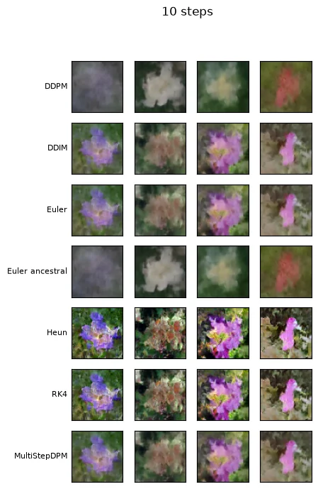

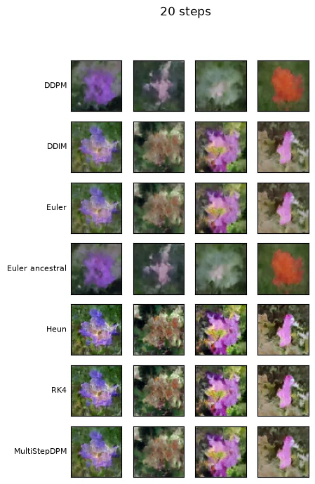
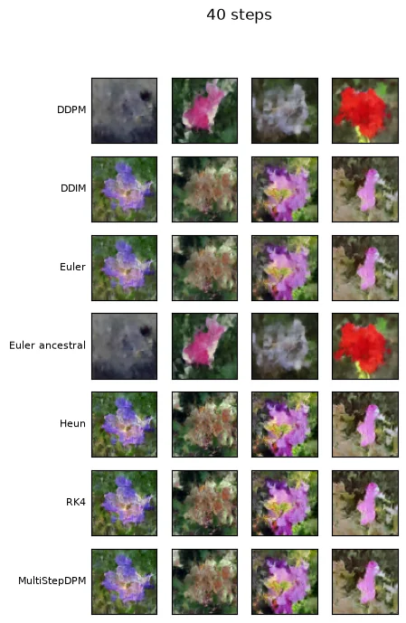
At 10 steps DDPM and Euler ancestral leave grey, unfinished images, because the fresh noise they add needs more steps to be removed. Heun and RK4 come out sharper and more contrasty than Euler at 10 steps. By 40 steps the deterministic samplers agree closely, and the two ancestral ones have found their own flowers.

Time per run

The time follows the number of model calls. At 40 steps RK4 takes about three times as long as Euler, and Heun a little under twice as long. At 10 steps each run takes only a few milliseconds, too short for this timer to separate the samplers well.

print(f"{'sampler':<16}" + "".join(f"{steps:>8} steps" for steps in STEP_COUNTS))
for name in SOLVERS:
    print(f"{name:<16}" + "".join(f"{seconds[name, steps] * 1000:>11.0f} ms" for steps in STEP_COUNTS))

sampler               10 steps      20 steps      40 steps
DDPM                      8 ms         12 ms         23 ms
DDIM                     11 ms         11 ms         21 ms
Euler                     6 ms         12 ms         22 ms
Euler ancestral          10 ms         11 ms         21 ms
Heun                     17 ms         18 ms         38 ms
RK4                      19 ms         35 ms         68 ms
MultiStepDPM              6 ms         11 ms         24 ms

How close the samplers get to each other

The deterministic samplers all solve the same ODE, so with enough steps they should land on nearly the same images. Below is the mean absolute pixel difference between each sampler’s images and Euler’s at 40 steps, on the [-1, 1] scale. The ancestral samplers add their own noise along the way, so they end up at different flowers. The last line compares the two ancestral samplers with each other: with the same key they give almost the same images, so on this schedule their updates nearly coincide.

reference = images["Euler", STEP_COUNTS[-1]]
for name in SOLVERS:
    difference = np.mean(np.abs(images[name, STEP_COUNTS[-1]] - reference))
    print(f"{name:<16} {difference:.4f}")
print("DDPM against Euler ancestral:", np.mean(np.abs(images["DDPM", STEP_COUNTS[-1]] - images["Euler ancestral", STEP_COUNTS[-1]])))

DDPM             0.3648
DDIM             0.0003
Euler            0.0000
Euler ancestral  0.3647
Heun             0.0406
RK4              0.0421
MultiStepDPM     0.0281
DDPM against Euler ancestral: 0.0004695011

Presets pair a training schedule with a sampling schedule

A sampler walks whatever noise levels the process gives it, and those have to match the ones the model trained on. That is why Dew keeps both in one Process. EDM trains on log-normal noise levels and samples on the Karras grid. The cosine preset trains and samples one discrete schedule with v-prediction. The flow preset is rectified flow on both sides. Sampling a model with a different process than it trained with walks the wrong path.

for name in ("edm", "karras", "cosine", "flow"):
    built = presets.build(name)()
    print(f"{name:<7} train: {type(built.schedule).__name__:<24} "
          f"sample: {type(built.sampler_schedule).__name__:<24} "
          f"predicts: {type(built.prediction).__name__}")

edm     train: EDMNoiseScheduler        sample: KarrasVENoiseScheduler   predicts: KarrasPredictionTransform
karras  train: KarrasVENoiseScheduler   sample: KarrasVENoiseScheduler   predicts: KarrasPredictionTransform
cosine  train: CosineNoiseScheduler     sample: CosineNoiseScheduler     predicts: VPredictionTransform
flow    train: FlowMatchingScheduler    sample: FlowMatchingScheduler    predicts: FlowMatchPredictionTransform

Where to go next

Notebook 03 adds a text caption and classifier-free guidance on top of the same sample call.